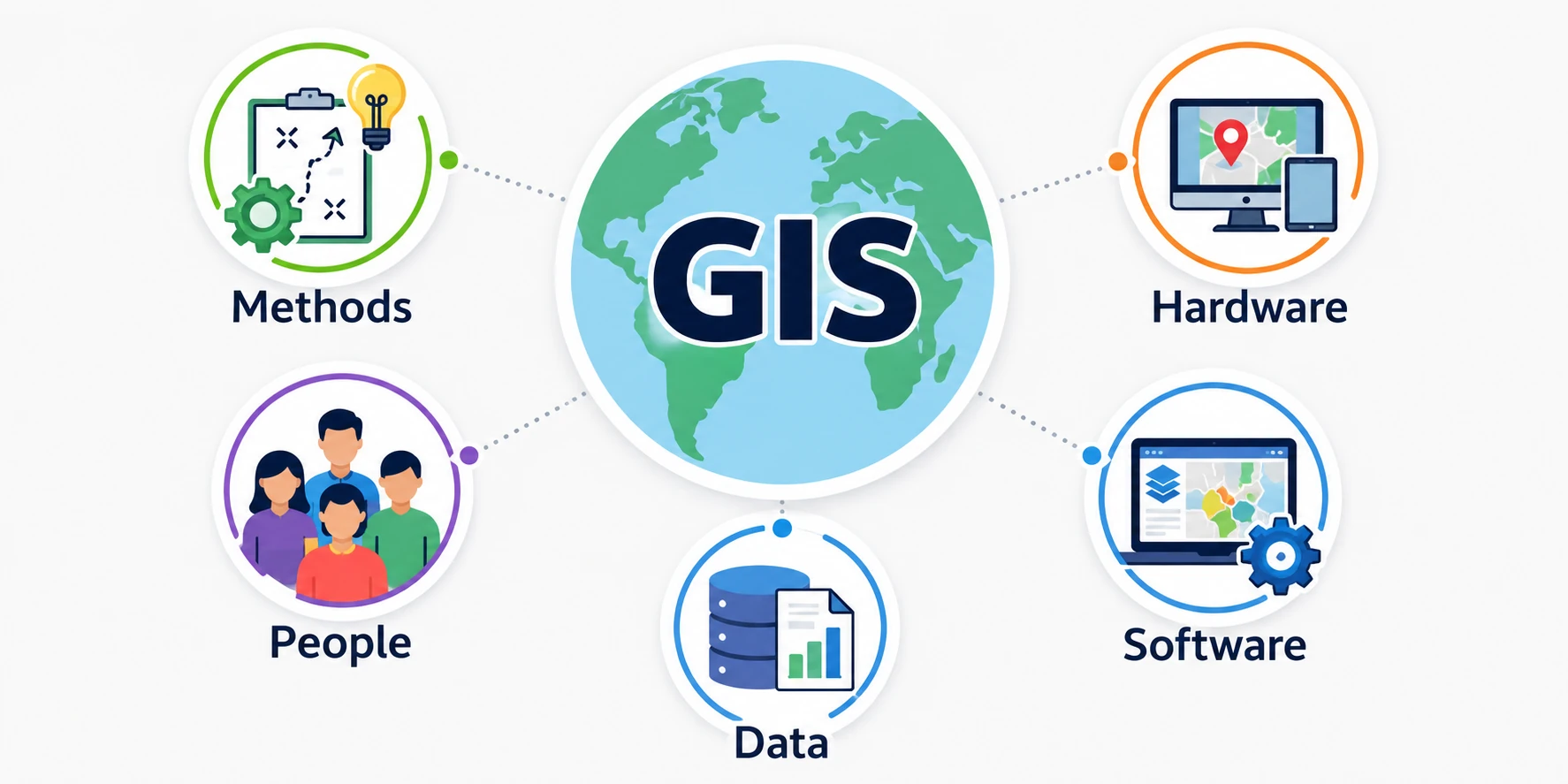
When we talk about GIS, we often immediately think about software. QGIS, ArcGIS, PostGIS, Python, libraries, plugins, geoalgorithms. All of this is useful, of course, but the real point, at least in the way I have always understood GIS, is not the software. The real point is the method we choose to read a phenomenon on the territory.
And this is where H3 comes into play! H3 is a geospatial indexing system developed by Uber. It allows us to divide the entire surface of the Earth into cells, mostly hexagonal, each one identified by a unique code. Said like this, it may sound very technical, almost something only for specialists, but the basic concept is very simple: we take the territory, we divide it into regular portions, and we use these portions as units of analysis.
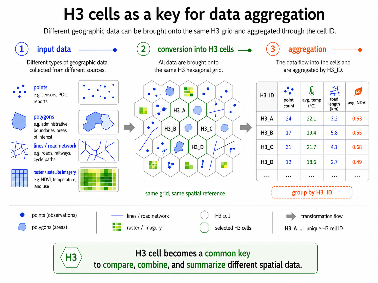
In practice, instead of comparing administrative polygons, census sections, urban areas, green areas, land use portions, or geometries that change in shape and size, we can bring everything back to a common grid.
And for those who work with geographic data, this is a real change of perspective!
Let’s take a step back. Anyone who has worked with territorial data knows very well that geographic data rarely arrives clean, homogeneous, and ready to be compared. Let’s think about ISTAT census sections (ISTAT is "Istituto Nazionale di Statistica" which produces and publishes all the official data and analyses regarding Italy's economy, society, and population). Within the same municipality, they can have very different shapes and sizes. If we compare different census years, the situation becomes even more complex because the geometries may change over time.
The same idea applies to many other territorial datasets. Corine Land Cover, for example, in its vector version, is made up of polygons with different shapes and sizes. These are very useful data, but they are not always easy to compare, especially when we want to read the evolution of a phenomenon over time.
So, the problem is methodological: how can I compare different areas if the starting spatial units are not homogeneous?
One possible answer is to use a grid. For years, we have been used to seeing square or rectangular grids, both in raster data and in many vector analyses. They are practical, easy to build, and intuitive. But they are not the only possible solution.
In many cases, hexagons work better! But why exactly hexagons?
The question is fair: why should I use a hexagonal grid instead of a normal square grid?
The first advantage is related to proximity.
In a square grid, each cell has side neighbours and diagonal neighbours. This means that not all neighbours are really “near” in the same way. Side squares share an edge, while diagonal squares share only one point.
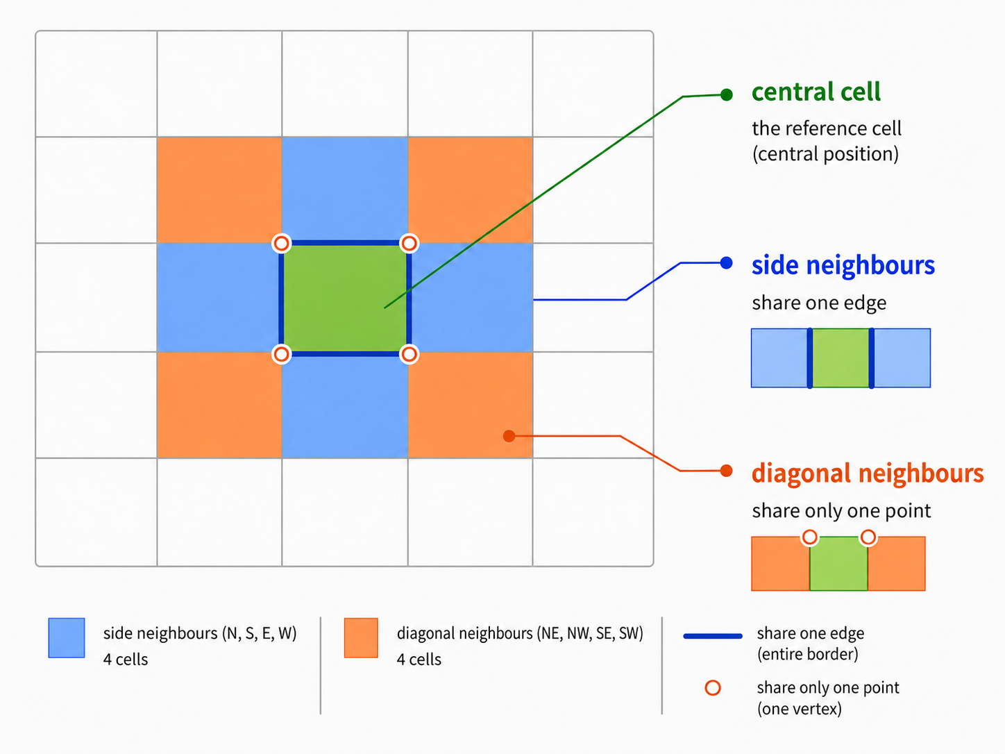
In a hexagonal grid, instead, each hexagon has six neighbours, and all of them share one edge. The relationship of proximity is more uniform.
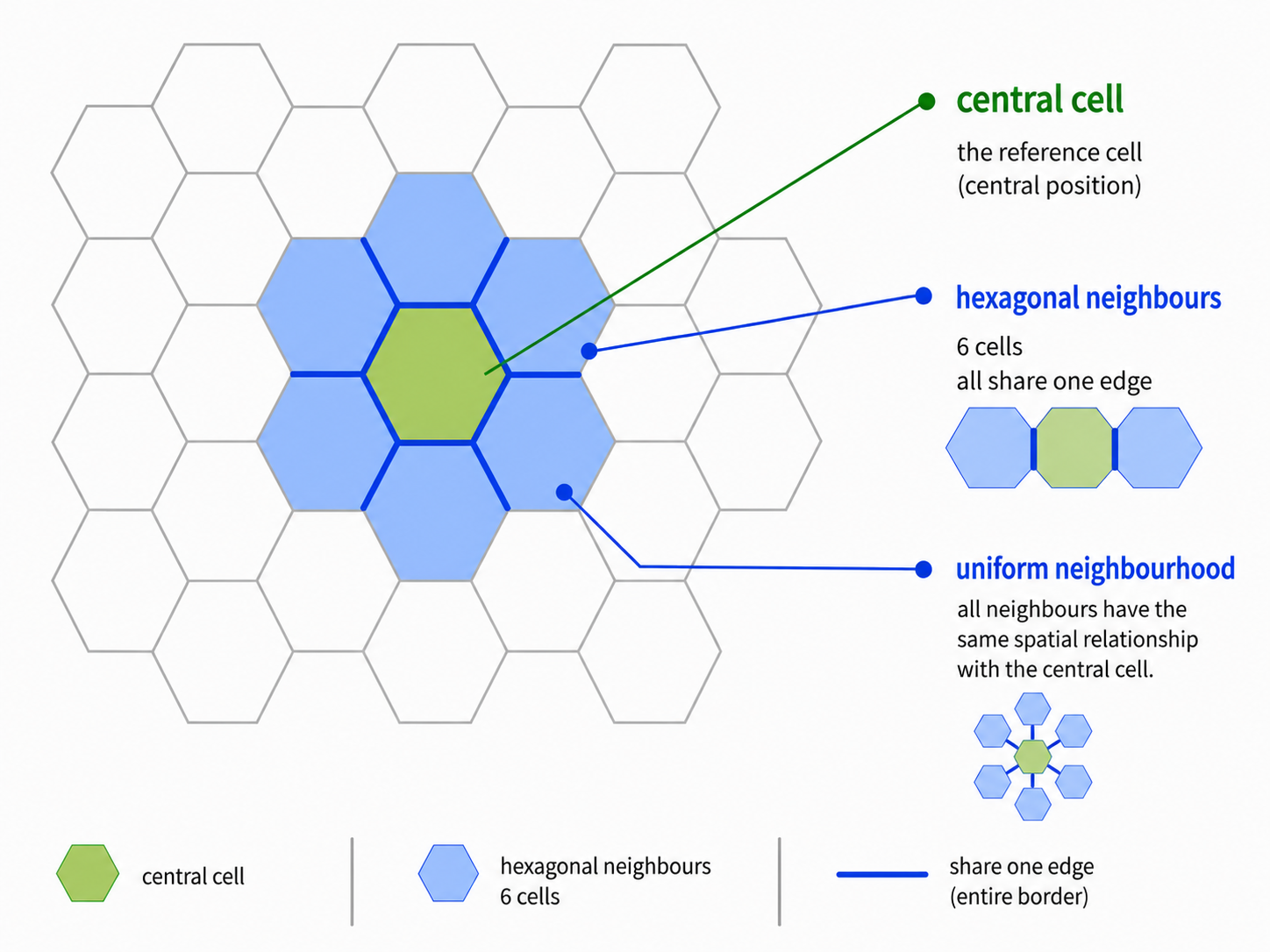
This may look like just geometry, but in reality it has very concrete effects in spatial analysis. If I am studying a phenomenon distributed in space — urban green areas, heat islands, flood risk, population density, accessibility to services, air quality — having cells with a more regular neighbourhood relationship helps me read spatial patterns better.
The second advantage is related to shape.
The hexagon approximates the circle better than the square. The circle is the shape that most naturally represents the idea of uniform distance from a centre. We cannot fill a plane only with circles without leaving empty spaces, but among the geometric shapes that can tile the space, the hexagon is one of the best approximations.
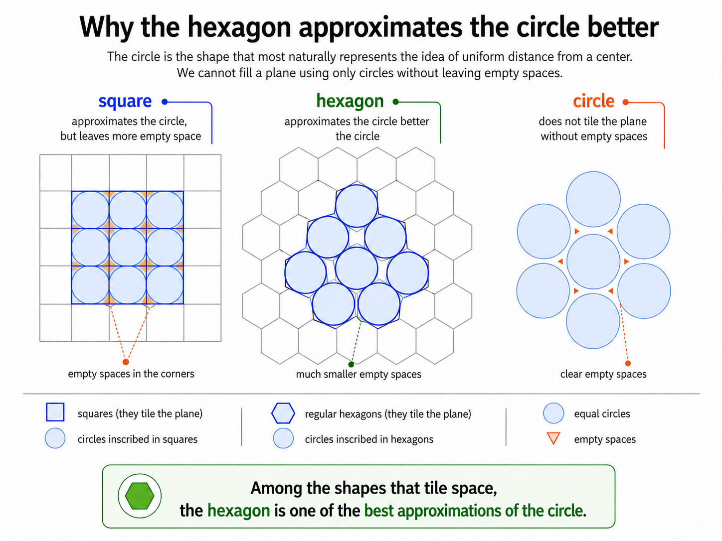
In other words: if I want to observe a phenomenon around a point, the hexagon gives me a more balanced representation than the square.
Till now, we have talked about hexagons in general. H3 takes one more step. It does not simply build a hexagonal grid over a single study area, but it creates a global, hierarchical, and indexed system. This means that each H3 cell has its own identifier and belongs to a specific resolution level.
The levels go from 0 to 15. At level 0, we have very large cells, useful for global or continental representations. As we move down through the levels, the grid becomes finer and finer. At the highest levels, we can reach very small cells, theoretically even smaller than one square metre. The system is hierarchical because I can move from a more detailed cell to a more general one, and vice versa. This is very interesting for multi-scale analysis: I can observe the same phenomenon at a regional, urban, neighbourhood, or micro-area scale simply by changing the grid resolution.
And it is indexed because each cell is not only a geometry, but also a key!
This is the game changer! When a cell becomes a key, I can use it in a database, in a table, in a Python process, in a PostGIS pipeline, in a data warehouse, or in a machine learning model. I can aggregate points, calculate statistics, compare different datasets, and build territorial indicators using a common spatial reference.
In practice, H3 transforms part of the spatial problem into a data organisation problem. And when there is a lot of data, this makes the difference!
At this point, there is an important detail. The Earth is not a plane and, as we know very well when we talk about cartography, reference systems, geoid, ellipsoid, and projections, representing the Earth’s surface is never an easiest operation.
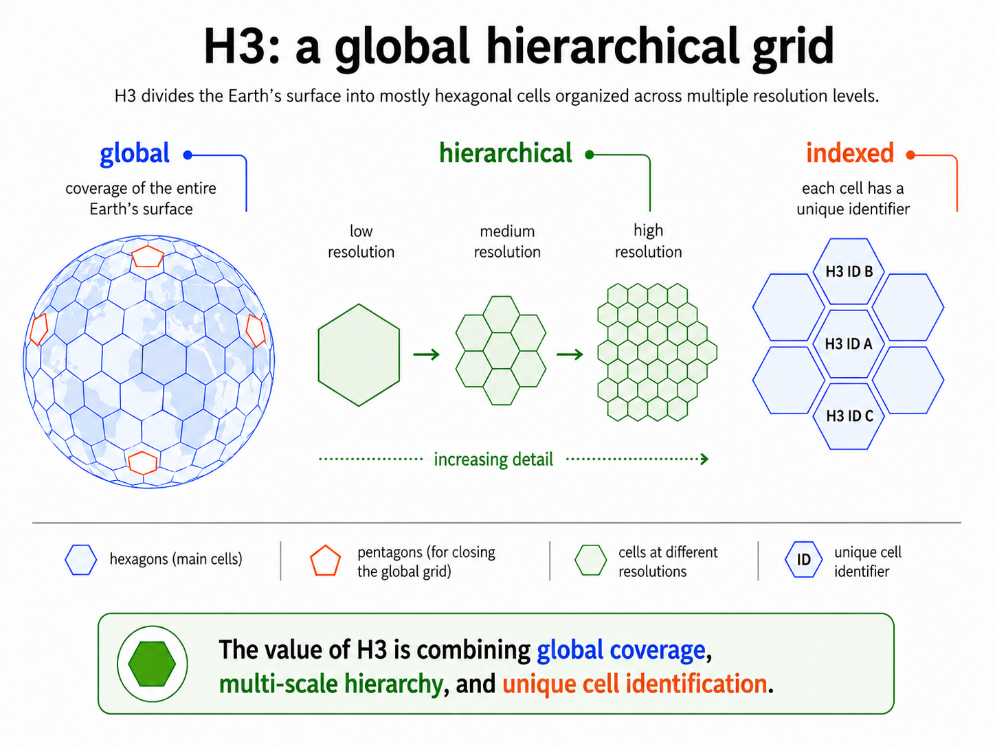
H3 builds its grid starting from an icosahedron circumscribed around the Earth’s sphere. The cells are generated on the faces of the icosahedron and then projected onto the Earth’s surface.
This allows us to have a global grid, but it also brings an inevitable consequence: it is not possible to tile a sphere using only perfect hexagons.
For this reason, at each H3 resolution there are also 12 pentagons. This is not an error, it is a geometric necessity. In most territorial analyses, these pentagons are not a practical problem, but it is important to know that they exist.
In the same way, it is important to remember that H3 cells do not all have exactly the same area. The average area is known for each resolution, but the real area can vary depending on the position of the cell in relation to the icosahedron.
So H3 is very useful, but it is not magic, it must be used knowing what we are doing.
Let me give you a concrete and real example, taken from an article I wrote some years ago with Giovanni Giacco and Luca Battisti, where we applied H3 to the study of urban green areas in the city of Turin.
The starting question was simple, but not trivial at all:
where would it be most useful to create new green areas inside the city?
To answer this question, we analysed the distribution of public green areas using three levels of the H3 grid: 7, 8, and 9.
At level 7, Turin was represented by a few dozen hexagons. The detail was more general, useful to read large areas and identify the first critical zones. At this scale, the areas with higher intervention priority appeared in the north-eastern part of the city, especially towards Regio Parco and Falchera.
Moving to level 8, the number of cells increased and the reading became more detailed. The critical areas did not disappear; on the contrary, they became clearer. Other areas started to emerge, such as Madonna di Campagna, Le Vallette, and Parella. At the same time, some first positive areas also appeared, such as San Donato. At level 9, the picture became even more interesting. There were many more cells, and the level of detail allowed us to observe clusters and hotspots that were less visible at the previous levels. In addition to the critical areas already identified, new priority areas appeared towards Nizza Millefonti and Mercati Generali, while in the Mirafiori Nord area we observed groups of cells in better conditions.
This is the most interesting point: when we change resolution, the phenomenon does not change. What changes is our ability to read it.
At a more general scale, we see the overall picture. At a finer scale, we begin to distinguish local differences better and this is exactly where H3 becomes useful for territorial planning.
But pay attention! H3 is a methodological tool. It does not replace rasters, it does not replace the original vector data, and it does not replace technical reasoning. It helps us build a common spatial structure on which we can aggregate, compare, and interpret data. It can simplify some analyses, make some phenomena easier to read, and help us build more comparable territorial indicators, but the original data remains fundamental.
If I have to calculate a real surface, interpret an administrative boundary, evaluate a cadastral geometry, analyse a DEM, or perform a precise spatial intersection, I still need classic GIS tools and the original geometries.
H3 comes into play when I want to observe a phenomenon through a regular, stable, and repeatable grid. In this sense, it is an excellent ally for environmental, urban, and territorial analyses.
And its possible applications are many. In environmental monitoring, H3 can be used to aggregate indices derived from satellite images, such as NDVI, NBR, or NDWI, and compare them with climate data, air quality data, or land use data.
In urban planning, it can help read the distribution of green areas, services, population, heat islands, or impermeable surfaces. In territorial risk analysis, it can be useful to build priority maps by combining data on floods, landslides, fires, population exposure, and building vulnerability. In geomarketing and mobility, it can be used to aggregate flows, movements, event density, or the distribution of points of interest.
The advantage is always the same: bringing different phenomena onto the same spatial structure.
In my opinion, the most interesting value of H3 is not only technical. The real value is in the possibility to compare.
Compare different areas at the same time. Compare the same area in different moments. Compare different phenomena on the same grid. Compare different scales without completely losing the link between the general level and the local level.
In a time when we have more and more territorial, satellite, climate, environmental, social, and economic data, the problem is no longer only having the data. The problem is being able to read it and to read it, we need a method.
H3 is one of those methods that can help us move from the map as a simple representation to the map as a tool for reasoning.
It is not enough to colour some hexagons on a map to make a good analysis, but if those hexagons are built with a clear method, if the data is solid, and if there is a clear question behind the analysis, then they can become a very effective way to understand where to intervene, with what priority, and with what objectives.
After all, this is exactly what a GIS should do: transform geographic data into useful knowledge for making better decisions.
What do you think?